This article was written solely for informational and educational purposes, and does not constitute medical advice. If you have any health concerns, please consult a qualified medical professional.
If I am screened for a disease and receive a positive test result, how worried should I be? What are the chances it was a false positive? In this article I’ll discuss why medical test results aren’t always as straightforward as they might seem, and how an equation first discovered over 200 years ago can help us to understand them better.
Sensitivity and Specificity
When interpreting a diagnostic test result, two of most important pieces of information we need to know are the sensitivity and specificity of the test. Coined in 1947 by Jacob Yerushalmy, these terms refer respectively to the probability that a diagnostic test will correctly identify someone with a disease, and the probability that it will accurately distinguish those without the condition.
Steven McGee gives a helpful illustration of these concepts in his book Evidence-Based Physical Diagnosis, using a hypothetical experiment. He asks us to imagine that a specific physical examination finding – a holosystolic heart murmur – is assessed in a group of 42 people with a particular type of valvular heart disease and a group of 58 people without the condition, producing the following results.
Physical Examination Findings in Patients With and Without Tricuspid Regurgitation
|
Valvular Heart Disease Status |
| Patients With Tricuspid Regurgitation |
Patients Without Tricuspid Regurgitation |
| Physical Examination Finding |
Holosystolic Murmur Present |
22 |
3 |
| Holosystolic Murmur Absent |
20 |
55 |
The sensitivity of a test for a disease is the proportion of patients who have the condition and test positive. To calculate it we can divide the number of true positives by the sum of the number of true positives and the number of false negatives.
- \(\text{FP}\) denotes the number of false positives.
- \(\text{FN}\) denotes the number of false negatives.
- \(\text{TP}\) denotes the number of true positives.
- \(\text{TN}\) denotes the number of true negatives.
For the example above this gives us a specificity of
\[
\text{Sensitivity}=\frac{\text{TP}}{\text{TP}+\text{FN}}=\frac{22}{22+20}=\frac{22}{42}\approx0.52,
\] equivalent to around 52%. We can find the specificity – the proportion of patients without the disease who correctly test negative – similarly;
\[
\text{Specificity}=\frac{\text{TN}}{\text{TN}+\text{FP}}=\frac{22}{55+3}=\frac{55}{58}\approx0.95.
\]
The Base Rate Fallacy
Now we’re clear on the definitions of sensitivity and specificity, let’s look at a common way in which these values can be misinterpreted. Imagine there is a medical condition, let’s call it Bayesitis, with a prevalence of 5% – meaning it affects one in 20 people. Now suppose that a blood test for Bayesitis is found to have a sensitivity of 99% and a specificity of 85%. If a random member of the population has their blood tested and receives a positive result, what is the probability that it is a false positive and they don’t actually have the disease?
We might intuitively assume that the answer is 15% since, according to the definition of specificity, this is the proportion of patients without Bayesitis who will test positive incorrectly. Unfortunately, by making this assumption, we are falling into the trap of the base rate fallacy.
Let’s see if we can get a ballpark figure for the true probability by thinking through what would happen if we were to screen a representative sample of 20 people for Bayesitis. We’ll assume that one person in our sample – 5% – has the disease. Since the sensitivity of our blood test is 99% this person is very likely to test positive, giving us one true positive. Now, what about the 19 people in our sample who do not have the disease? Referring to the specificity of our blood test, we can expect it to correctly identify 85% percent of them, giving us 16.15 true negatives. Since we can’t have 0.15 of a person, let’s round this to 16, which leaves us with three false positives.

So three out of four positive test results from our representative sample are false, meaning that if someone from our sample receives a positive test result, the probability that they don’t actually have Bayesitis is 75%. This is far enough from our initial guess of 15% for us to know that we must have made an error in our reasoning.
Our problem was that we failed to take into account the population prevalence, or base rate, of Bayesitis. To see the importance of the base rate, consider a group of people in which 0% have the condition – in a population like this, there is a 100% probability that any positive test results are false.
Clearly, the sensitivity and specificity of a test aren’t on their own sufficient for us to calculate the probability that any particular positive test result is false. How, then, do we find the exact value of this probability?
Bayes to the Rescue
The answer, of course, is Bayes’ Theorem. Discovered by Thomas Bayes in the 1740s century, and given its modern form by Pierre Simon Laplace in 1812, this famous theorem states that for any two events \(A\) and \(B\), we can get the conditional probability of \(A\) given \(B\) from the conditional probability of \(B\) given \(A\) using the formula
\[
\mathbb{P}(A|B)=\frac{\mathbb{P}(B|A)\mathbb{P}(A)}{\mathbb{P}(B)},
\]
where \(\mathbb{P}(A)\) and \(\mathbb{P}(B)\) are the marginal (unconditional) probabilities of \(A\) and \(B\) respectively.
In our example, \(A\) corresponds to the event that the person who had their blood tested actually has Bayesitis, and \(B\) corresponds to the event that they test positive for the disease. When we committed the base rate fallacy, we made the mistake of assuming that \(\mathbb{P}(A|B)\) was equivalent to \(\mathbb{P}(B|A)\), and we failed to consider the marginal probabilities \(\mathbb{P}(A)\) and \(\mathbb{P}(B)\). Let’s try to work out the probability that their test result was a false positive again, this time using Bayes’ theorem.
- \(D^{-}\) denotes not having the disease.
- \(D^{+}\) denotes having the disease.
- \(T^{-}\) denotes testing negative.
- \(T^{+}\) denotes testing positive
We want to find
\[
\mathbb{P}(D^{-}|T^{+})=\frac{\mathbb{P}(T^{+}|D^{-})\mathbb{P}(D^{-})}{\mathbb{P}(T^{+})}.
\]
We know that \(\mathbb{P}(D^{-})=0.95\), equivalent to 95%, since the prevalence of Bayesitis in the population is 95%. We also know \(\mathbb{P}(T^{+}|D^{-})=0.15\), as we defined our imaginary test to be 85% accurate. So to find the probability of a positive test result being false we just need to find the denominator of the fraction above; \(\mathbb{P}(T^{+})\), the overall probability of testing positive.
We can write
\[
\begin{split}
\mathbb{P}(T^{+})&=\mathbb{P}(T^{+}\cap(D^{+}\cup D^{-}))
\\&=\mathbb{P}(T^{+}\cap D^{+})+\mathbb{P}(T^{+}\cap D^{-})
\\&=\mathbb{P}(T^{+}|D^{+})\mathbb{P}(D^{+})+\mathbb{P}(T^{+}|D^{-})\mathbb{P}(D^{-}),
\end{split}
\] using the fact that \(D^{+}\) and \(D^{-}\) are collectively exhaustive and mutually exclusive events, as well as the definition of conditional probability, which we can rearrange to get that \(\mathbb{P}(A\cap B)=\mathbb{P}(A|B)\mathbb{P}(B)\).
Now, to work out \(\mathbb{P}(T^{+})\), we can use our knowledge of the sensitivity and specificity of our blood test and the prevalence of Bayesitis to subsitute in the values \(\mathbb{P}(T^{+}|D^{+})=0.99\), \(\mathbb{P}(D)=0.05\), \(\mathbb{P}(T^{+}|D^{-})=0.15\), and \(\mathbb{P}(D^{-})=0.95\), finding that
\[
\mathbb{P}(T^{+})=0.99\times 0.05 + 0.15\times 0.95 = 0.192.
\]
Finally, we can calculate that
\[
\mathbb{P}(D^{-}|T^{+})=\frac{0.15\times0.95}{0.192}=0.7421875,
\]
which is pretty close to the estimate we got from our thought experiment involving 20 people!
To check our answer, we can use R to simulate repeatedly sampling 20 people from a population of 1 million people with a 5% prevalence of Bayesitis.
Simulating Bayesitis Screening in R
# Because we will be using randomly generated numbers, we first set a seed to ensure our results are reproducible:
set.seed(31415926)
# We now set up some variables:
pop_size <- 1000000
bayesitis_prevalence <- 0.05
bayesitis_pop_size <- pop_size * bayesitis_prevalence # we calculate 5% of the population to find the number of people that have Bayesitis
# Now imagine that each person in the population is assigned a number randomly pick 5% of these numbers to designate the people that have Bayesitis
total_pop <- 1:pop_size # we create a vector made up of the numbers from 1 to 1,000,000
bayesitis_pop <- sample(total_pop, size=bayesitis_pop_size, replace=FALSE) # we randomly samples 5% of the entries from our total_pop vector
# Let's create a logical vector (one that only contains TRUE and FALSE values) to represent the Bayesitis status of every member of the population:
bayesitis_statuses <- rep(FALSE, times=pop_size) # we initialise a vector the length of the population where every entry is FALSE
bayesitis_statuses[bayesitis_pop] <- TRUE # we change the entries corresponding to the people with Byesitis to TRUE
# We can now set up our simulations:
num_sims <- 300
false_pos_props <- rep(NA, times=num_sims) # we initialise a vector to store the proportion of false positives we get from each simulation
# Now let's repeatedly pick 20 random people from the population and simulate screening them for Bayesitis:
samp_size <- 20
for (n in 1:num_sims) {
rand_samp <- sample(total_pop, size=samp_size, replace=FALSE)
# Let's set up variables to store the number of true and false positive test results:
num_true_pos <- 0
num_false_pos <- 0
rand_nums <- runif(samp_size, min=0, max=1) # we generate 20 random numbers between 0 and 1, so that everyone in the sample gets a correct/incorrect
# test result with a probability according to the sensitivity and specificty of our test
for (i in 1:samp_size) {
true_status <- bayesitis_statuses[rand_samp[i]]
if (rand_nums[i] <= 0.99 & true_status == TRUE) { # if the person does have Bayesitis they get an accurate positive result with a probability of 99%
num_true_pos <- num_true_pos + 1
} else if (rand_nums[i] > 0.85 & true_status == FALSE) { # if they don't they get a false positive result with a probability of 15%
num_false_pos <- num_false_pos + 1
}
}
total_pos <- num_true_pos + num_false_pos
if (total_pos != 0) { # if there are no positive test results, true or false, the proportion of positive test results that are false is undefined
false_pos_props[n] <- num_false_pos / total_pos
}
}
# Now let's see how the average proportion of positive test results that are false changes as the number of simulations we've done increases:
props_for_avg <- false_pos_props[!is.na(false_pos_props)] # we remove the undefined values from our vector of empirical false positive probabilities
cum_avg <- cumsum(props_for_avg) / seq_along(props_for_avg) # we calculate a cumulative average as the number of simulations increases
# We plot the cumulative average against the number of simulations:
par(mar=c(bottom=4.2, left=5.1, top=1.8, right=0.9), family="Roboto Slab")
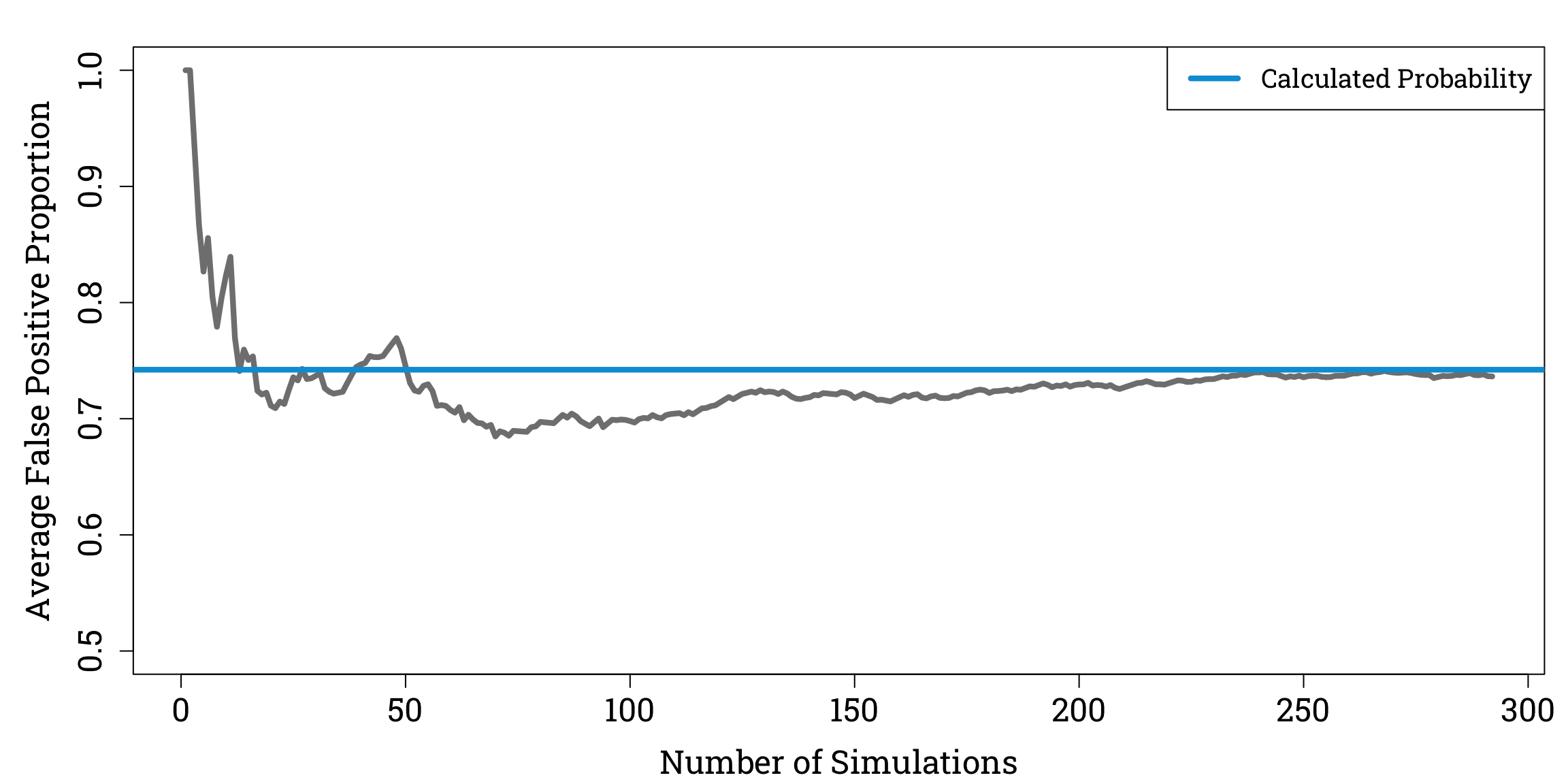
plot(cum_avg, ylim=c(0.5,1), xlab="Number of Simulations", ylab="Average False Positive Proportion", type="l", col="#808080", lwd=4.2, cex.lab=1.5, cex.axis=1.5)
abline(h=0.7421875, col="#009ed8", lty=1, lwd=4.2)
legend("topright", legend="Calculated Probability", col="#009ed8", lty=1, lwd=4.2, cex=1.2)
Reassuringly, as we do more simulations, the average proportion of positive test results that are false appears to converge to our calculated value of \(\mathbb{P}(D^{-}|T^{+})\).