This article was written solely for informational and educational purposes, and does not constitute medical advice. If you have any health concerns, please consult a qualified medical professional.
Imagine you are experiencing a medical problem, and your doctor suggests you try a new drug treatment. You’re curious about how much evidence there is to suggest that this treatment will work for you, so you do some research and find out that it has been tested in eight clinical trials. Two of them found that the drug was more effective than a placebo, but six of them did not show a significant benefit – meaning the results could reasonably have occurred even if the treatment had no effect. You feel somewhat concerned that three quarters of the papers published on this new treatment regime failed to prove its worth. On the other hand, you notice that the two positive results came from the studies with the largest sample sizes, which you are inclined to think makes them more reliable. Taking all the evidence into account, what conclusions should you draw?
Weighing Up the Evidence
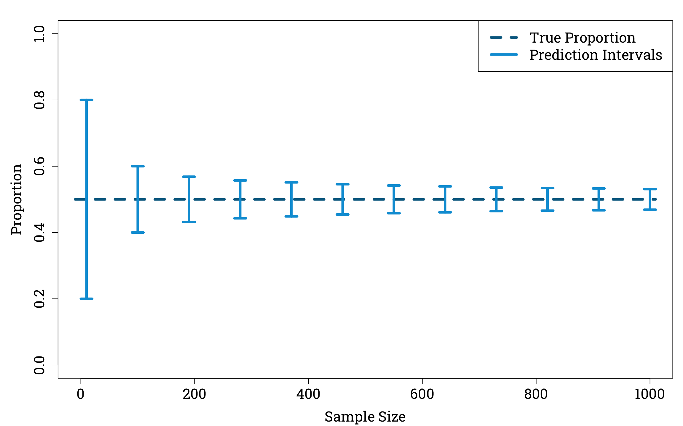
We all intuitively feel that estimates calculated using larger sample sizes are more trustworthy than those arrived at from tiny fractions of the population. For example, if you saw the hyperbolic newspaper headline ‘Britain Prefers Cats to Dogs!’ and then read in the article that this conclusion was based on six out of a sample of ten people saying they prefer cats, you’d likely be a lot more sceptical than if you read that it was based on 600 out of a sample of 1000 people preferring cats.
We can examine this example using the binomial distribution. If the true proportion of the population that prefer cats to dogs is 50%, then we can calculate that if we randomly sample 1000 people from the population there is only a 5% probability that the amount of people who prefer cats in our sample will be either smaller than 469 or greater than 531. In other words, if the true proportion of the population that prefer cats to dogs, \(p\), is equal to 0.5, the 95% prediction interval for \(\hat{p}\), our estimate of the true proportion based on a random sample of 1000 people, is (0.469,0.531). If we only sample 10 people, on the other hand, this interval widens considerably, to (0.2,0.8).
Plotting Binomial Prediction Intervals in R
true_p <- 0.5
samp_sizes <-  seq(10, 1000, by=90) # creating a vector of twelve equally spaced sample sizes from 10 to 1000
alpha <- 0.05
lower_95s <- qbinom(alpha/2,
                   samp_sizes,
                   true_p)/samp_sizes
upper_95s <- qbinom(1-alpha/2,
                   samp_sizes,
                   true_p)/samp_sizes
par(mar=c(bottom=4.2, left=5.1, top=1.8, right=0.9), family="Roboto Slab") # setting the plot options
plot(c(-10, 1010), c(true_p, true_p),
     xlab = "Sample Size", ylab = "Proportion",
     xlim=c(0,1000), ylim=c(0,1),
     type="l", lty=2,
     lwd=4.2, col="#006a90",
     cex.lab=1.5, cex.axis=1.5)
for (i in 1:length(samp_sizes)) {
  samp_size <- samp_sizes[i]
  upper <- upper_95s[i]
  lower <- lower_95s[i]
  segments(x0=samp_size-10, y0=lower,
           x1=samp_size+10, y1=lower,
           lwd=4.2, col="#009ed8")
  segments(x0=samp_size-10, y0=upper,
           x1=samp_size+10, y1=upper,
           lwd=4.2, col="#009ed8")
  segments(x0=samp_size, y0=upper,
           x1=samp_size, y1=lower,
           lwd=4.2, col="#009ed8")
}
legend("topright", # adding a key
       legend=c("True Proportion ", "Prediction Intervals "), lty=c(2,1),
       col=c("#006a90","#009ed8"), lwd=4.2, cex=1.5)
Smaller sample sizes naturally introduce greater variance into our estimator of the true proportion.
Now let’s return to the scenario in which we want to combine the results of multiple trials. How can we do this in a principled way whilst taking into account the varying levels of precision in the estimates of the treatment’s effect produced by different trials?
In medical research, formal procedures known as meta-analyses are often used to statistically combine evidence from all the randomised controlled trials of a tratment that have been conducted. In the rest of this article, I’ll work through the steps of a fixed-effect meta-analysis – the simplest kind of meta-analysis, in which we assume that all the research is measuring the same true effect and that any variations in results arise solely from sampling error – using data from an early and influential systematic review.
Antenatal Steroids
In 1972, an obstetrican and neonatologist working at the National Women’s Hospital in Auckland, New Zealand, published the initial findings from a randomised contolled trial they had begun in 1969. Once all the results were in, this trial showed a significant reduction in the mortality of premature babies whose mothers had been given antenatal steroids, compared to those whose mothers had not received this treatment.
However, one unreplicated trial rarely provides enough evidence for medical practice to change drastically. Over the following decade, another seven trials of this treatment were carried out (all with smaller sample sizes), but only two of them showed an effect that was statistically significant at a significance level of 5%. It took a later meta-analysis to show that, when combined, the first eight RCTs of antenatal steroids were in fact sufficient to show a significant effect of antenatal steroids on neonatal mortality in premature babies.
The results of all eight of these studies can be found in a Cochrane review from 1996.
Inputting the Results of the Eight RCTs into a Data Frame in R
steroid_trials <- data.frame(
  control_group_size = c(538, 61, 59, 71, 75, 58, 63, 372),
  control_group_deaths = c(60, 5, 7, 10, 7, 12, 11, 34),
  treatment_group_size = c(532, 69, 67, 56, 71, 64, 81, 371),
  treatment_group_deaths = c(36, 1, 3, 8, 1, 3, 4, 32))

trial_names <- c("Liggins and Howie (1972)",
                 "Block et al. (1977)",
                 "Morrison et al. (1978)",
                 "Taeusch et al. (1979)",
                 "Papageorgiou et al. (1979)",
                 "Schutte et al. (1979)",
                 "Doran et al. (1980)",
                 "Collaborative Group (1981)")

rownames(steroid_trials) <- trial_names
steroid_trials$total_trial_size <- with(steroid_trials, control_group_size + treatment_group_size)
num_trials <- nrow(steroid_trials)
The Results of the First Eight Randomised Controlled Trials of the Effect of Antenatal Steroids on Neonatal Mortality in Premature Babies
|
Control Group |
Treatment Group |
Total
Number of
Babies in the Study |
Number of
Babies in the
Group |
Number of
Neonatal Deaths |
Number of
Babies in the
Group |
Number of
Neonatal Deaths |
| Randomised Control Trial |
Liggins and Howie
(1972) |
538 |
60 |
532 |
36 |
1070 |
Block et al.
(1977) |
61 |
5 |
69 |
1 |
130 |
Morrison et al.
(1978) |
59 |
7 |
67 |
3 |
126 |
Taeusch et al.
(1979) |
71 |
10 |
56 |
8 |
127 |
Papageorgiou et al.
(1979) |
75 |
7 |
71 |
1 |
146 |
Schutte et al.
(1979) |
58 |
12 |
64 |
3 |
122 |
Doran et al.
(1980) |
63 |
11 |
81 |
4 |
144 |
Collaborative Group
(1981) |
372 |
34 |
371 |
32 |
743 |
Here, the years in parentheses after the authors’ names are the years of publication of the first papers they disseminated relating to their trials. The table is organised chronologically according to the order in which these papers were published.
The Individual Trials’ Findings
Once all the eligible trials have been identified and assessed for bias, the first step of any meta-analysis is to estimate a treatment effect from each of them.
In this article, we will use the risk ratio as a measure of the treatment effect. This is a common measure of the association between an exposure and an event, and is equal to the probability of the event in the exposed group divided by the probability of the event in the non exposed group.
For example, suppose that a trial produces the following contingency table.
Example Contingency Table
|
Intervention Group |
Control Group |
| Number of Events |
\(a\) |
\(c\) |
| Number of Non-Events |
\(b\) |
\(d\) |
Then we can find an estimate for the risk ratio using the formula
\[
\widehat{\text{RR}}=\frac{a}{a+b}\div\frac{c}{c+d}.
\]
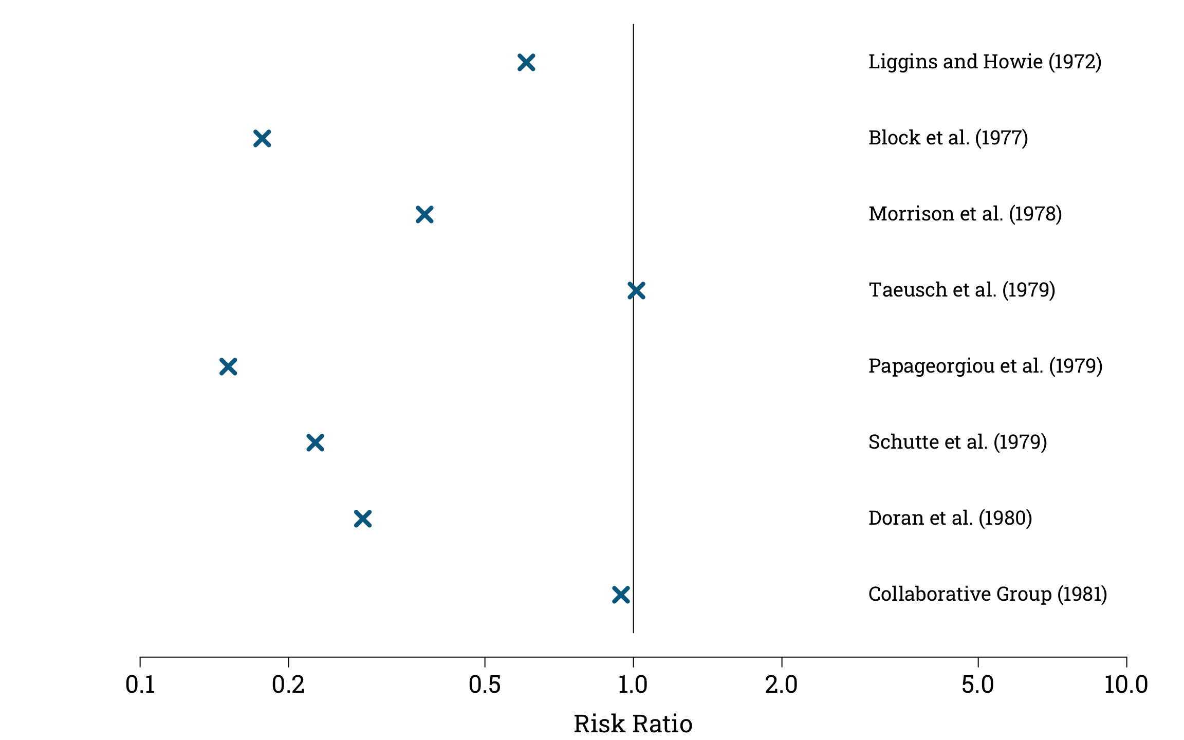
A risk ratio of \(1\) indicates that there is no difference in the probability of the event occurring in the exposed group and the probability of the event occurring in the non-exposed group. Risk ratios are usually plotted on a logarithmic scales in forest plots, so that a change in risk ratio representing a doubling in risk appears equal to a change in risk ratio representing a halving of risk.
Calculating and Plotting the Risk Ratios in R
steroid_trials$risk_ratio <- with(steroid_trials,
                                  (treatment_group_deaths/treatment_group_size)
                                  / (control_group_deaths/control_group_size))

empty_results_plot <- function (xax, yax) { # creating a function we can call again to set up an empty plot
                                            # on which to display the results of the different trials
  plot(1, type="n", log = "x",
     cex.lab=1.5, cex.axis=1.5,
     xlim=xax, xlab="Risk Ratio",
     ylim=yax, ylab=" ", frame.plot = FALSE, yaxt="n")
  yline <- yax + c(-0.5, 0.5)
  segments(1, yax[1], 1, yax[2])
  for (i in 1:num_trials) {
    y_coord <- num_trials+1-i
    text(3, y_coord, adj=0, trial_names[i], cex=1.2)
  }
}

par(mar=c(bottom=4.2, left=5.1, top=0, right=0.9), family="Roboto Slab") # setting the plot options
empty_results_plot(xax=c(0.1, 10), yax=c(0.5, 8.5))
points(steroid_trials$risk_ratio, 8:1,
       pch=4, col="#006a90", cex=1.8, lwd=4.2)
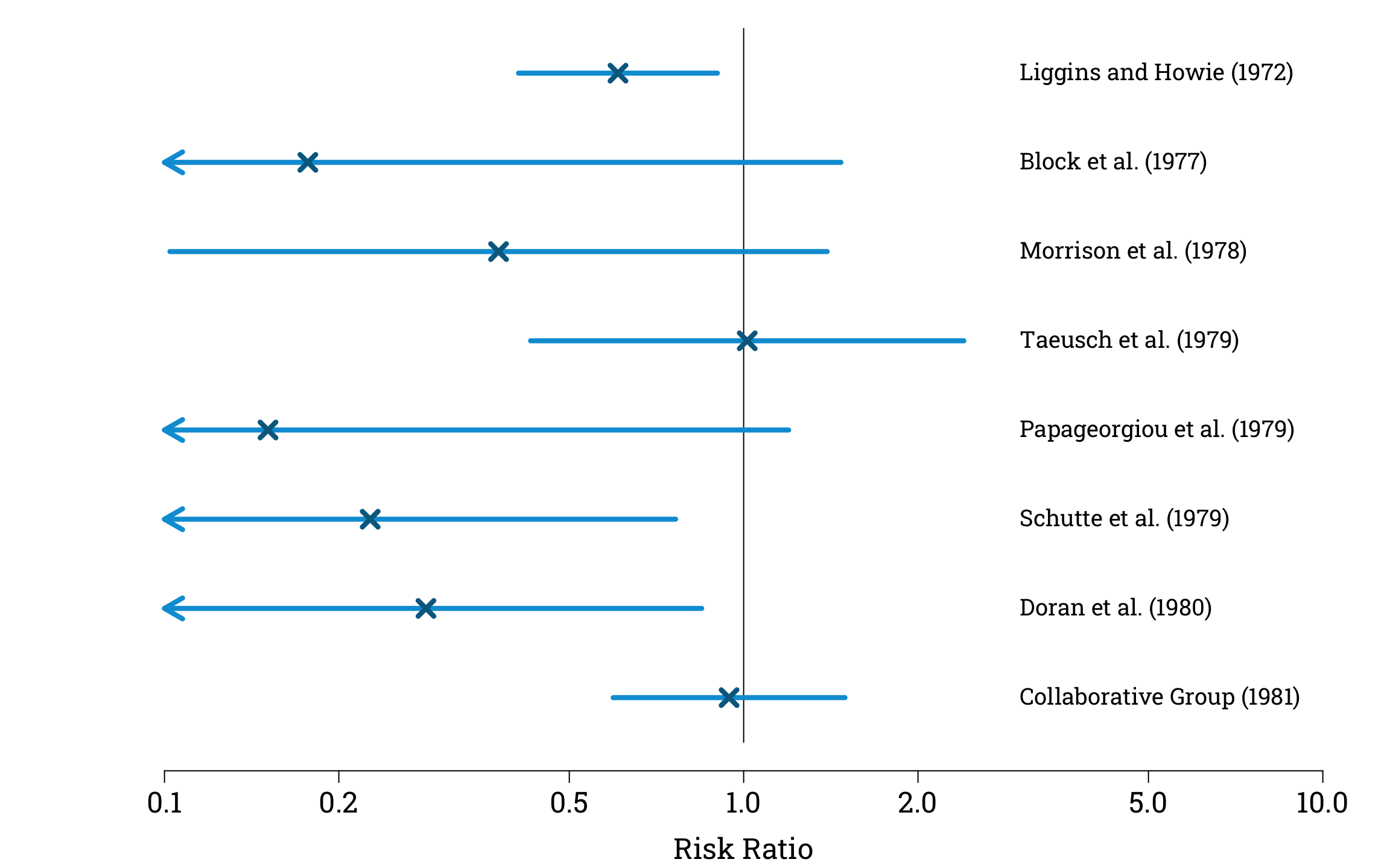
These point estimates for the risk ratio are not very useful on their own, because they do not give information about the different levels of uncertainty surrounding each estimate.
To solve this problem, we can calculate approximate 95% confidence intervals for each study, using the fact that the natural logarithm of our estimator of the risk ratio converges in distribution to a normal distribution with a mean of zero, and a variance that we can estimate using the formula
\[
\text{Var}(\text{log}\widehat{\text{RR}})=\frac{1}{a}-\frac{1}{a+b}+\frac{1}{c}+\frac{1}{c+d},
\]
where \(a\), \(b\), \(c\), and \(d\) again represent the counts in the contingency table.
Estimating and Plotting the Confidence Intervals in R
confidence_intervals <- data.frame(
  lower = rep(NA, times=num_trials),
  upper = rep(NA, times=num_trials)
)
alpha <- 0.05
z_val <- qnorm(1-alpha/2)
confidence_intervals$lower <- with(steroid_trials,
                                   exp(
                                     log(risk_ratio)
                                     - z_val * sqrt(1/treatment_group_deaths - 1/treatment_group_size
                                                    + 1/control_group_deaths - 1/control_group_size)
                                   ))
confidence_intervals$upper <- with(steroid_trials,
                                   exp(
                                     log(risk_ratio)
                                     + z_val * sqrt(1/treatment_group_deaths - 1/treatment_group_size
                                                    + 1/control_group_deaths - 1/control_group_size)
                                   ))

par(mar=c(bottom=4.2, left=5.1, top=0, right=0.9), family="Roboto Slab")
empty_results_plot(xax=c(0.1, 10), yax=c(0.5, 8.5))

plot_CIs <- function(CIs_df) {
  num_CIs <- nrow(CIs_df)
  for (i in 1:num_CIs){
    y_coord <- num_CIs+1-i
    lower <- CIs_df$lower[i]
    upper <- CIs_df$upper[i]
    if (lower < 0.1) {
      arrows(x0=0.1, y0=y_coord,
             x1=upper, y1=y_coord,
             code=1, length=0.18,
             lwd=4.2, col="#009ed8")
    } else {
      segments(x0=lower, y0=y_coord,
               x1=upper, y1=y_coord,
               lwd=4.2, col="#009ed8")
    }
  }
}

plot_CIs(confidence_intervals)
points(steroid_trials$risk_ratio, 8:1,
       pch=4, col="#006a90", cex=1.8, lwd=4.2)
Pooling the Results
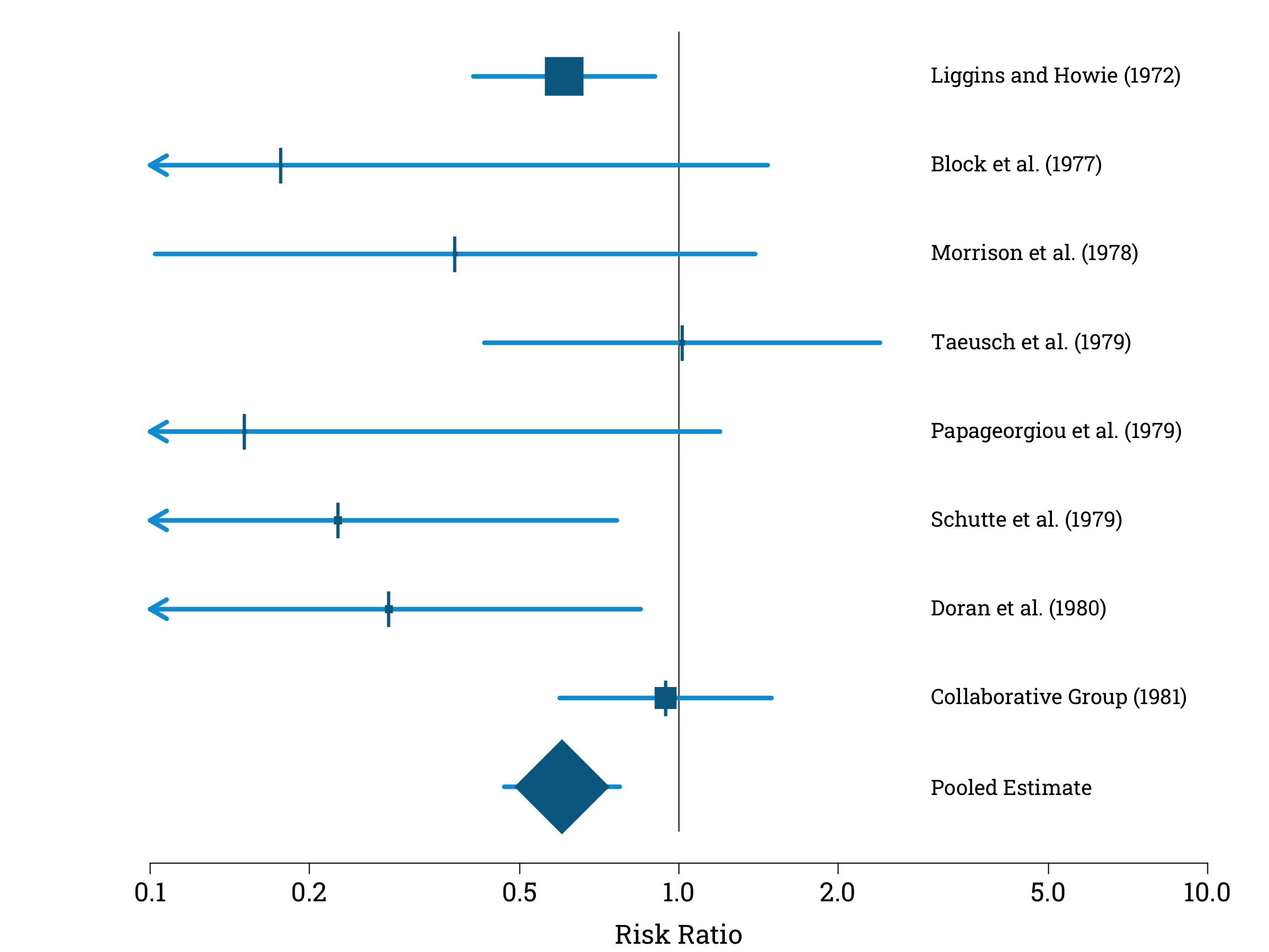
Now we want to combine these estimates, giving more weight to the those with lower variance. One way to do this would be to give each estimate a weight proportional to the inverse an estimate of its variance, which we could calculate using our previously estimated standard deviation of the log risk ratio. However, this method can be unreliable when the study size is small or the probability of the event we are studying is rare, which is why the Cochrane Collaboration recommends that researchers use the Mantel-Haenszel method for pooling estimates instead.
In this method, each estimate, \(\widehat{\text{RR}}_i\), is given a weight of
\[
w_i=\frac{(a_i+b_i)c_i}{a_i+b_i+c_i+d_i},
\]
where for each trial \(a_i\) and \(b_i\) are the numbers of events and non-events in the exposed group, and \(c_i\) and \(d_i\) are the numbers of the events and non-events in the non-exposed group. The Mantel-Haenszel estimate is then equal to
\[
\widehat{\text{RR}}_{\text{MH}}=\frac{\sum w_i \widehat{\text{RR}}_i}{\sum w_i}.
\]
We can find an approximate confidence interval for the Mantel-Haenszel estimator using the asmpymptotic normality of its natural logarithm. An approximation for its variance is
\[
\text{Var}(\text{log}\widehat{\text{RR}}_{\text{MH}})=\frac{P}{RS},
\]
with \(P\), \(R\), and \(S\) defined by the formulae
\[
\begin{split}
P&=\sum_i\frac{(n_{1i}n_{2i}(a_i+c_i)-a_ic_iN_i)}{N_i^2},\\
R&=\sum_i\frac{a_in_{2i}}{N_i},\\
S&=\sum_i\frac{c_in_{1i}}{N_i}.
\end{split}
\]
- \(a_i\), \(b_i\), \(c_i\), and \(d_i\) denote the contingency table counts of trial \(i\).
- \(n_{1i}=a_i+b_i\) and \(n_{2i}=c_i+d_i\) denote the sizes of the treatment and control groups in trial \(i\).
- \(N_i=n_{1i}+n_{2i}\) denotes the total size of trial \(i\).
Calculating a Mantel-Haenszel Pooled Estimate and Confidence Interval for the First Eight Antenatal Steroid RCTs in R
weights <- with(steroid_trials, treatment_group_size * control_group_deaths / total_trial_size)
steroid_trials$normalised_weight <- weights / sum(weights)
pooled_rr_estimate <- sum(steroid_trials$risk_ratio * steroid_trials$normalised_weight)

n_1 <- steroid_trials$treatment_group_size
n_2 <- steroid_trials$control_group_size
a <- steroid_trials$treatment_group_deaths
c <- steroid_trials$control_group_deaths
N <- steroid_trials$total_trial_size
P <- sum((n_1*n_2*(a+c)-a*c*N)/N^2)
R <- sum(a*n_2/N)
S <- sum(c*n_1/N)
log_SE <- sqrt(P/(R*S))

alpha <- 0.05
z_val <- qnorm(1-alpha/2)
log_CI_lower <- log(pooled_rr_estimate) - z_val * log_SE
log_CI_upper <- log(pooled_rr_estimate) + z_val * log_SE
CI <- exp(c(log_CI_lower, log_CI_upper))
cat("M-H Risk Ratio Estimate: ", pooled_rr_estimate,
    ",\n95% Confidence Interval: (", exp(log_CI_lower), ", ", exp(log_CI_upper), ")", sep = "")
M-H Risk Ratio Estimate: 0.6009549,
95% Confidence Interval: (0.4673707, 0.7727203)
Our final pooled estimate for the risk ratio is 0.60 to 2 significant figures. This is equivalent to a 40% reduction in the risk of neonatal death in premature babies whose mothers had been given antenatal steroids.
To complete our visualisation of the results of our meta analysis, let’s add our Mantel-Haenszel estimate and its confidence interval to our plot. This produces a summary graphic known in the literature as a forest plot. By convention, we plot the individual estimates using squares with sizes proportional to their weights, and use a diamond to distinguish our pooled estimate.
Creating the Final Forest Plot in R
par(mar=c(bottom=4.2, left=5.1, top=0, right=0.9), family="Roboto Slab")
empty_results_plot(xax=c(0.1, 10), yax=c(-0.5, 8.5))
text(3, 0, adj=0, "Pooled Estimate", cex=1.2)

plot_CIs(confidence_intervals)
segments(x0=CI[1], y0=0,
         x1=CI[2], y1=0,
         lwd=4.2, col="#009ed8")

sizes <- steroid_trials$normalised_weight*12
points(steroid_trials$risk_ratio, 8:1,
       pch=15, col="#006a90", cex=sizes, lwd=4.2)
points(steroid_trials$risk_ratio, 8:1,
       pch="|", col="#006a90", cex=2.4)
points(pooled_rr_estimate, 0, pch=18, col="#006a90", cex=12)
A meta-analysis of these eight trials, and several more completed in the intervening years, was eventually published in a systematic review in 1989. This systematic review led directly to the publication of new guidelines by the Royal College of Obstetricians and Gynaecologists in 1992, and antenatal steroids are now routinely given to mothers in premature labour. Their use is monitored, as a measure of optimal perinatal care, in the National Neonatal Audit Programme run by the Royal College of Paediatrics and Child Health. The 1989 systematic review also inspired the Cochrane Collaboration’s logo – to learn more, see this page on their website.